Human rights stats, part 2
My previous post promised some simulations. To refresh your memory, I am trying to see how reliably Multiple Systems Estimation, as described here, can guess the true number of fish in a pond.
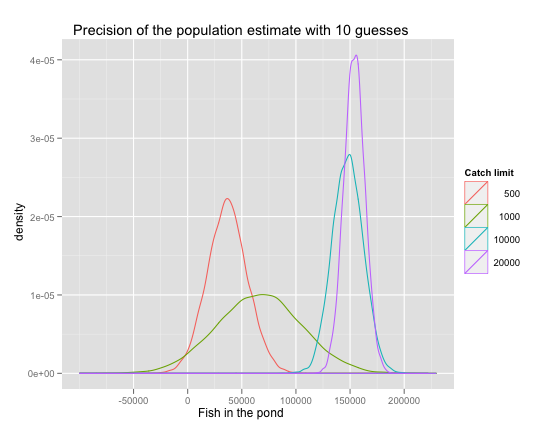
The density plot below tells the story. The true number of fish is 150,000. Each catch limit lets you make a best guess, which is the x-coordinate of the peak of its associated bell curve. The shape of each bell curve measures the uncertainty surrounding the guess: the flatter the bell, the more uncertain the guess. Perfect foresight would be a spike at the 150,000 x-mark. Curves that peak away from that mark make biased guesses.
It is obvious that larger daily catch limits allow you to guess better. Very low catch limits set you up for severe downward bias. The red curve, corresponding to a daily catch of up to 500 fish, cannot help underestimating the true population size, for reasons discussed in the previous post. Then there seems to be a range of catch limits that improve on the bias, but increase the uncertainty horribly – that’s the green curve. So, you need higher limits, but you don’t have to go crazy. The gain in precision after some point is not worth it: though a limit of 20,000 is very accurate, a limit of half that is not much worse.
I was inspired to run this exercise by a class I’m taking. The work would have been slower without help from here (I recommend the book, I bought it) and here. The picture would not have looked this good without ggplot2 (you should get that book too). All errors are my own. Here’s the code:
# http://www.foreignpolicy.com/articles/2012/02/27/the_body_counter?page=full
# simulate MSE = Multiple Systems Estimation

# SOME HOUSEKEPING FIRST

# pretty picture comes from here
library("ggplot2")

# true population size
population <- 150000

# number of guesses you can take to estimate
# maximum-likelihood mean, standard deviation
# of your final guess
n <- 10

# this many draws will help you simulate
# the uncertainty of your guess
sims <- 10^4

# define a function that will render big numbers with comma
# separators for thousands. the original version is here:
# https://stat.ethz.ch/pipermail/r-help/2010-November/259488.html
commaUS <- function(x) {
   sprintf("%s", formatC(x, format="fg", big.mark = ","))
}

# THE PIECES OF THE ACTUAL SIMULATION

# make one guess, with daily catches of up to x:
# -- if x=100, the daily catch is between 0 and 99
# -- if x=1000, the daily catch is between 0 and 999.
mymse <- function(x) {
   day1 <- round(runif(1)*x)       # count of fish caught on day 1
   day2 <- round(runif(1)*x)       # count of fish caught on day 2
   pond <- c(1:population)
   day1 <- sample(pond,day1)               # list of fish caught on day 1
   day2 <- sample(pond,day2)               # list of fish caught on day 2
   overlap <- length(intersect(day1,day2)) # count of fish caught twice
   guess <- length(day1)*length(day2)
   if(overlap>0) {
      guess <- guess/overlap
   }
   return(round(guess))
}

# assume that the fish population guesses for a given pond
# are distributed N(mu,sigma). this is the log likelihood
# function of a given set of y guesses:
myll <- function(par, y) {
   mu <- par[1]
   sigma <- par[2]
   l <- length(y)*log(sigma^2)
   a <- 1/sigma^2
   ll <- sum((y-mu)^2)
   return(-(l+a*ll)/2)
}

# collect n guesses of catches limited to
# a given maxcatch, then estimate mu, sigma
# and make sims draws from N(mu, sigma)
mysim <- function(n,maxcatch) {
   # 1. make n guesses of fish in the pond
   a <- apply(as.matrix(1:n),1,function(x) mymse(maxcatch))
   # 2. get the maximum likelihood estimates of mu, sigma
   # that might have produced the n guesses:
   opt <- optim(par=c(1,1), fn = myll, control = list(fnscale = -1),
          y=a, method = "BFGS", hessian = TRUE)
   # 3. model the uncertainty around these estimates
   return(rnorm(sims,mean=opt$par[1],sd=opt$par[2]))
}

# THE FINAL PICTURE

# now make some comparisons of the effect of
# maxcatch with a given number of guesses n
# on the population estimate and its precision
maxes  <- c(500,1000,10000,20000)

simspic <- matrix(0,sims,length(maxes))
for(i in 1:length(maxes)) {
   simspic[,i] <- mysim(n,maxes[i])
}

# Set up a stacked 2-column matrix where the second
# column will be used for grouping these guesses
x.1 <- cbind(simspic[,1],maxes[1])
x.2 <- cbind(simspic[,2],maxes[2])
x.3 <- cbind(simspic[,3],maxes[3])
x.4 <- cbind(simspic[,4],maxes[4])

# now plot the guesses with the
# catch limits set in maxes
d <- as.data.frame(rbind(x.1,x.2,x.3,x.4))
p <- qplot(V1, colour=factor(V2), data=d, geom="density", xlab="Fish in the pond")
t <- paste("Precision of the population estimate with",n,"guesses",sep=" ")
p <- p + scale_colour_discrete(name = "Catch limit") + opts(title=t)
p
If you made it here, you might also want to see one last thing on the matter.