Human rights stats, one last thing
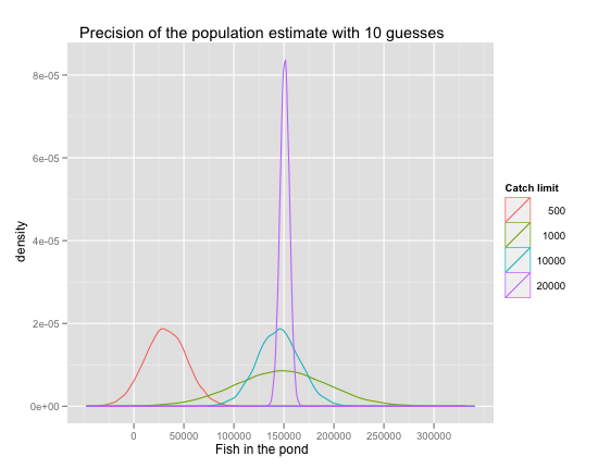
The R code in my previous post could also produce the picture below. The implication is this:
A small sample is still bad news. It is biased toward underestimating the population. There’s nothing you can do about that. The larger the sample, the better. How large a sample do you need? You might get lucky with as little as 1,000, for the reason that I mentioned in my first installment on the topic: small samples only need a small overlap to guess pretty well. That’s why the green curve now peaks at the true population mark. But you’d have to be lucky, as my previous picture demonstrates by counter-example. And even a correct guess will be surrounded by a lot of uncertainty if you have a small sample: the green curve is still the flattest of the three that guess correctly. Finally, the gain from increasing the catch limit from 10,000 to 20,000 is not trivial after all: the purple curve is quite a bit peakier than the blue one.
What this simulation shows is that MSE relies on having representative samples of the true population. There’s no way out of that requirement. You also want to run your code more than once. Though you will be able to dismiss easily sample sizes that are clearly too small, there may be a range of sample sizes that can provide false comfort. I could have easily seen this picture first and concluded that 1,000 isn’t great, but it still hits the mark, so maybe it’s good enough. That would have been wrong. On the other hand, now I’m pretty sure that 10,000 is still alright, though not as good as it looked before.